Build a neural network from scratch in PyTorch — then let PyTorch do the work
The best way to understand deep learning is to build a small network by hand — forward pass, loss, backpropagation and gradient descent — and then rebuild it the idiomatic PyTorch way. A beginner-friendly, code-first walkthrough.
 Nasir Mollah
5 min read
On this page9 sections
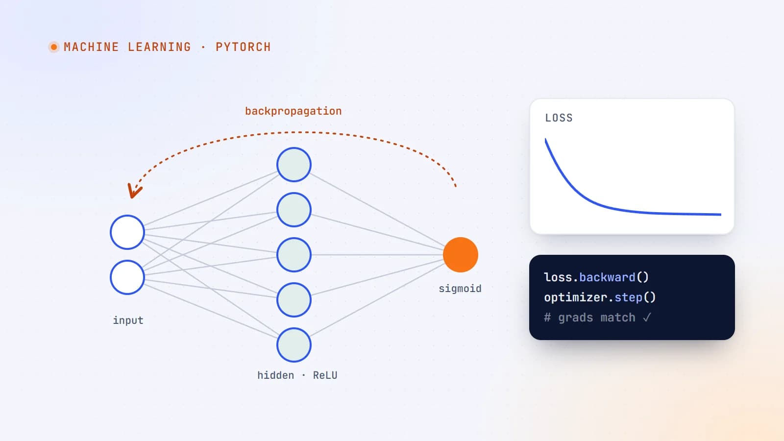
Deep learning frameworks make training a neural network look like three lines of code: loss.backward(), optimizer.step(), repeat. That’s wonderful for productivity — and terrible for understanding. When training goes wrong, you need to know what those lines actually do.
In this walkthrough we’ll build a small neural network completely by hand in PyTorch — including backpropagation, without autograd — then check our gradients against PyTorch’s, and finally rebuild the same model the idiomatic way. All you need is Python and PyTorch installed.
The problem: classify points
We’ll create a simple dataset: 2D points belonging to two clusters, labeled 0 and 1. The network’s job is to predict the label from the coordinates.
import torch

torch.manual_seed(0)

n = 200
X0 = torch.randn(n, 2) + torch.tensor([-2.0, -2.0])   # class 0, centered at (-2, -2)
X1 = torch.randn(n, 2) + torch.tensor([2.0, 2.0])     # class 1, centered at (2, 2)

X = torch.cat([X0, X1])                                 # shape (400, 2)
y = torch.cat([torch.zeros(n), torch.ones(n)]).unsqueeze(1)  # shape (400, 1)
The network
A small fully connected network:
- input: 2 numbers (the coordinates);
- hidden layer: 8 neurons with ReLU activation;
- output: 1 number turned into a probability with the sigmoid function.
Mathematically, for a batch of inputs X:
z1 = X · W1 + b1        (400×2)·(2×8) → (400×8)
a1 = ReLU(z1)
z2 = a1 · W2 + b2       (400×8)·(8×1) → (400×1)
p  = sigmoid(z2)        probability of class 1
W1, b1, W2, b2 are the parameters we need to learn.
W1 = torch.randn(2, 8) * 0.5
b1 = torch.zeros(8)
W2 = torch.randn(8, 1) * 0.5
b2 = torch.zeros(1)
Small random starting weights break the symmetry between neurons; if they all started equal, they’d all learn the same thing.
The loss: how wrong are we?
For binary classification we use binary cross-entropy:
loss = −mean( y·log(p) + (1−y)·log(1−p) )
It’s small when the network assigns high probability to the correct class and grows quickly when it’s confidently wrong.
def forward(X):
    z1 = X @ W1 + b1
    a1 = torch.relu(z1)
    z2 = a1 @ W2 + b2
    p = torch.sigmoid(z2)
    return z1, a1, p

def bce(p, y, eps=1e-7):
    p = p.clamp(eps, 1 - eps)        # avoid log(0)
    return -(y * torch.log(p) + (1 - y) * torch.log(1 - p)).mean()
Backpropagation by hand
To improve the parameters we need the gradient of the loss with respect to each one: how much the loss changes if we nudge that parameter. Backpropagation computes these with the chain rule, working backwards from the loss.
A convenient result: for sigmoid followed by binary cross-entropy, the gradient with respect to z2 simplifies to (p − y), divided by the batch size because we took the mean.
def backward(X, y, z1, a1, p):
    N = X.shape[0]
    dz2 = (p - y) / N                 # (400, 1)
    dW2 = a1.T @ dz2                  # (8, 1)
    db2 = dz2.sum(dim=0)              # (1,)

    da1 = dz2 @ W2.T                  # (400, 8)
    dz1 = da1 * (z1 > 0).float()      # ReLU passes gradient only where z1 > 0
    dW1 = X.T @ dz1                   # (2, 8)
    db1 = dz1.sum(dim=0)              # (8,)
    return dW1, db1, dW2, db2
Each line applies the chain rule one step further back. Notice how the shapes always match the parameters they belong to — a useful sanity check when you write this yourself.
Gradient descent
Now we repeatedly run the forward pass, compute gradients and move each parameter a small step against its gradient:
lr = 0.5

for epoch in range(300):
    z1, a1, p = forward(X)
    loss = bce(p, y)
    dW1, db1, dW2, db2 = backward(X, y, z1, a1, p)

    W1 -= lr * dW1
    b1 -= lr * db1
    W2 -= lr * dW2
    b2 -= lr * db2

    if epoch % 50 == 0:
        accuracy = ((p > 0.5).float() == y).float().mean()
        print(f"epoch {epoch:3d}  loss {loss:.4f}  accuracy {accuracy:.2%}")
The loss drops quickly and accuracy approaches 100% — these clusters are easy to separate. You’ve just trained a neural network with nothing but matrix multiplication and calculus.
Checking our gradients against autograd
How do we know the hand-written gradients are right? PyTorch’s autograd can compute them for us. We recreate the parameters with requires_grad=True and compare:
params = [t.clone().requires_grad_(True) for t in (W1, b1, W2, b2)]
aW1, ab1, aW2, ab2 = params

p_auto = torch.sigmoid(torch.relu(X @ aW1 + ab1) @ aW2 + ab2)
bce(p_auto, y).backward()

# manual gradients at the same parameter values
z1, a1, p = forward(X)
manual = backward(X, y, z1, a1, p)

for m, a in zip(manual, params):
    print(torch.allclose(m, a.grad, atol=1e-6))   # True, True, True, True
If all four print True, your backpropagation is correct. This gradient check is a great habit whenever you implement something by hand.
The idiomatic PyTorch version
Now that you know what happens underneath, here’s the same model the way you’d write it in practice:
import torch.nn as nn

model = nn.Sequential(
    nn.Linear(2, 8),
    nn.ReLU(),
    nn.Linear(8, 1),          # outputs logits (no sigmoid here)
)

loss_fn = nn.BCEWithLogitsLoss()     # sigmoid + BCE, numerically stable
optimizer = torch.optim.SGD(model.parameters(), lr=0.5)

for epoch in range(300):
    logits = model(X)
    loss = loss_fn(logits, y)

    optimizer.zero_grad()     # clear old gradients
    loss.backward()           # autograd computes every gradient
    optimizer.step()          # update every parameter

with torch.no_grad():
    accuracy = ((model(X) > 0).float() == y).float().mean()
print(f"accuracy {accuracy:.2%}")
Every line maps to something you built by hand:
nn.Linearholds a weight matrix and bias, likeW1/b1.BCEWithLogitsLosscombines the sigmoid and cross-entropy in one numerically stable step.loss.backward()does what ourbackwardfunction did — for any architecture.optimizer.step()is theW -= lr * dWupdate, and optimizers like Adam add smarter step sizes.optimizer.zero_grad()is needed because PyTorch accumulates gradients by default.
Scaling up: datasets, batches and GPUs
Real datasets don’t fit in one tensor operation, and real training uses mini-batches. PyTorch’s Dataset and DataLoader handle this:
from torch.utils.data import TensorDataset, DataLoader

device = "cuda" if torch.cuda.is_available() else "cpu"
model = model.to(device)

loader = DataLoader(TensorDataset(X, y), batch_size=32, shuffle=True)

for epoch in range(20):
    for xb, yb in loader:
        xb, yb = xb.to(device), yb.to(device)
        loss = loss_fn(model(xb), yb)
        optimizer.zero_grad()
        loss.backward()
        optimizer.step()
For images you’d write a custom Dataset that loads and transforms files, use convolutional layers (nn.Conv2d) instead of only linear ones, and add a separate validation set to detect overfitting.
What to take away
- A neural network is layers of matrix multiplications and non-linear activations.
- The loss measures how wrong the predictions are.
- Backpropagation applies the chain rule backwards to get every parameter’s gradient.
- Gradient descent nudges parameters against their gradients, over and over.
- PyTorch’s autograd, modules and optimizers automate exactly these steps — and knowing what they do makes debugging real models far easier.
The same ideas, scaled up enormously, power large language models — see how LLMs actually work. Try changing the hidden layer size, the learning rate or the dataset (for example, make the clusters overlap) and watch how training behaves. Building intuition with small, fully understood experiments is the fastest way to get good at deep learning.
- Machine Learning
- PyTorch
- Deep Learning
- Python
Keep reading
9 min read
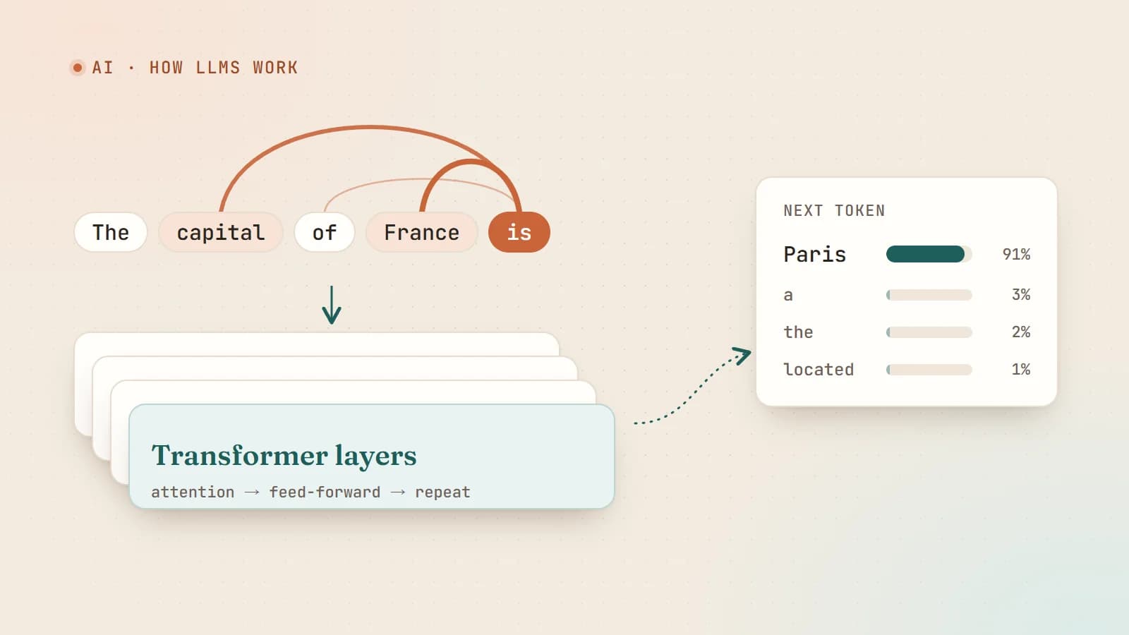
How large language models actually work — a plain-English guide for developers
Tokens, embeddings, attention, training and sampling — what really happens between your prompt and the model’s answer, explained without the hype and without a math degree.
- AI
- LLMs
- Machine Learning
- Fundamentals
5 min read
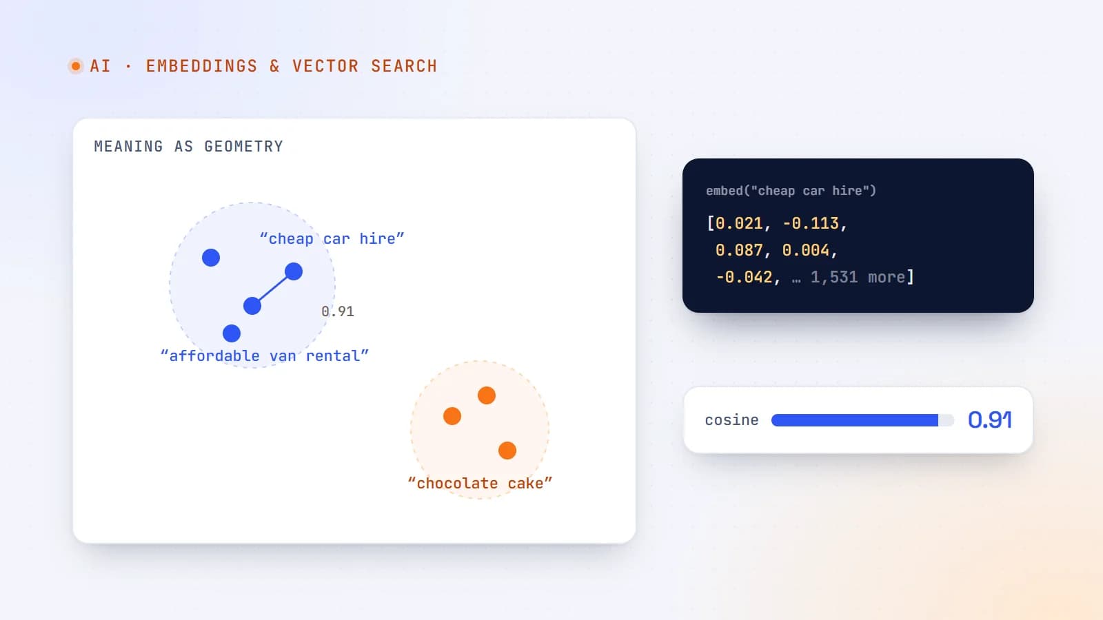
Embeddings and vector databases, explained for web developers
Embeddings turn text, images and products into lists of numbers that capture meaning — the technology behind semantic search, recommendations and RAG. Here’s how they work and how to use them in a real app.
- AI
- Embeddings
- Vector Search
- Machine Learning

5 min read
Google’s September 2026 spam update is done: how to check if your site was hit
Google’s fourth spam update of 2026 took almost 14 days to roll out — far longer than the others. Here’s a simple Search Console check to see if your traffic was affected, what spam policies usually trip up small business sites, and how to recover.
- SEO
- Google Updates
- Search Console
- Small Business
Building something? Let’s talk.
If you’re planning a web app, a website or a new feature, a free call is a good place to start — you’ll get honest options, a fixed price and a timeline.